Modeling Point Cloud Distortions in Mobile Laser Scanning for Surveying

Singh, Aman Kumar; Lohani, Bharat

doi:10.1061/JSUED2.SUENG-1663

★ Editor's Choice · Journal of Surveying Engineering

Modeling Point Cloud Distortions in Mobile Laser Scanning for Surveying

Aman Kumar Singh Bharat Lohani

Department of Civil Engineering, Indian Institute of Technology Kanpur

Journal of Surveying Engineering (ASCE), Vol. 152, No. 3, 04026006, 2026

Paper Thesis Slides Poster Try the simulator

Top and side views of a mobile mapper scanning a moving box. The box is drawn at three times t1, t2 and t3; the scanned length is shorter than the actual length, and the top and side faces of the scanned box come out as parallelograms. — **Where the distortion comes from.** A tilted profile scanner on a mobile mapper (pink) hits the moving box (blue) at different instants t₁, t₂, t₃. Each point is recorded where the box was at that instant, so the scanned length differs from the actual length, and the top (a) and side (b) faces come out as parallelograms.

Overview

A moving object never looks the way it is

A mobile laser scanner builds its point cloud one profile at a time. If the object being scanned is moving too, every profile catches it in a different place, and the cloud shows a shape that never existed.

Earlier studies noticed these distortions, but no one had described what kinds there are or written down the equations that govern them. This work does both. It classifies motion-induced distortions in mobile laser scanning (MLS) into two families, derives closed-form equations for each, and checks the equations against simulated LiDAR data.

Length

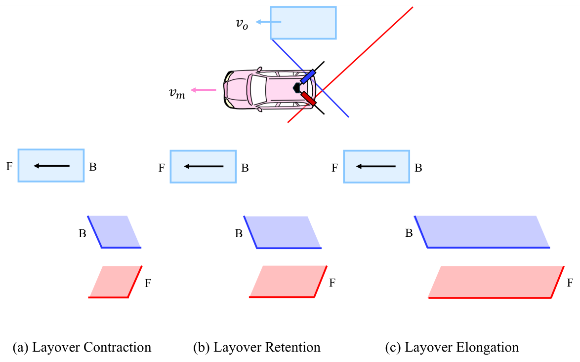
Shorter or longer

Head-on traffic shrinks; traffic you overtake stretches. The ratio depends only on two speeds.

Layover

Back where the front is

When the object outruns the scan line, its back is recorded first, and the cloud is flipped end to end.

Parallelepiped

Boxes become skewed

A tilted scan plane catches each face at a slant, so a cuboid turns into a parallelepiped with tilts γ, β and α.

Abstract

Mobile Laser Scanning (MLS) LiDAR data are susceptible to distortions when the scanned objects are in motion. Although some prior studies have acknowledged the existence of such distortions, there is yet no fundamental work describing their nature and types, and modeling them in the form of closed-form equations. This research, for the first time, systematically studies these distortions in detail and derives the fundamental equations governing them. The distortions are classified into two primary types: length distortion and parallelepiped distortion. Length distortion causes the point clouds of moving objects to appear shorter or longer than their actual sizes, depending on the relative direction of motion between the mobile mapper and the object. Another notable length distortion observed is layover, where the rear of a moving object appears in place of its front in the scanned point cloud. Parallelepiped distortion transforms the point cloud of a cuboid-shaped object into a skewed parallelepiped. The skew of the faces depends on the relative orientation between the scanning plane and the movement directions of the mobile mapper and the object. The derived equations have been verified through simulation. This deeper understanding of motion-induced point cloud distortions will contribute to more accurate analysis and interpretation of MLS data in dynamic environments.

Learn

The idea in five steps

No background in LiDAR is needed for this part. If you know that distance equals speed times time, you can follow it.

The scanner draws one line at a time

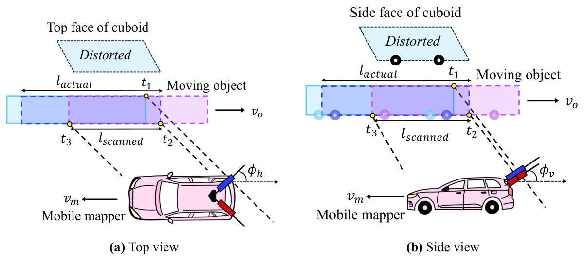
Survey-grade mobile mappers often carry 2D profile scanners. Each one spins a laser inside a single plane and records one thin slice of the world per rotation. The vehicle's own motion pushes that plane forward, and the slices stack up into a 3D point cloud.

The plane is usually tilted: turned by a horizontal angle φ_h away from straight sideways, and tipped by a vertical angle φ_v. Two scanners, left and right, cover both sides of the road.
For a still world, this works perfectly

GNSS and an inertial unit record where the scanner was at every instant. Each point is placed using the scanner's pose at the moment it was measured. A parked car comes out at its true size, because it was in the same place the whole time.
A moving object is in a different place for every slice

The scanner captures the front of a moving car at one moment and its back a fraction of a second later. In between, the car moved. The system still places each point correctly for that instant, but stitched together, the points describe a car that never existed.

Ego-motion compensation cannot fix this. It removes the scanner's motion, not the object's.
It is a race between the scan line and the object

Picture where the scan plane cuts the object's path. As the mapper drives, that cut point slides along the path at a speed v_l, which depends on the mapper's speed and the angles. The object moves along the same path at v_o. Compare the two:
- Head-on (they move toward each other): the scan finishes the object quickly. Contraction.
- The scan line overtakes the object (v_l > v_o): the scan has to chase it. Elongation.
- Same speed (v_l = v_o): the line rides along with one slice of the object forever. Over-elongation, a streak.
- The object outruns the line (0 < v_l < v_o): the back is captured first. Layover: front and back swap.
A slanted plane makes the box lean

Because the scan plane is tilted, the near and far edges of a face are not captured at the same instant either. The object moves in between, so every face shears into a parallelogram. The top face tilts by γ, the side faces by β, and together they push the front and back faces off square by α. The box becomes a parallelepiped.

Top: a mobile mapper with red and blue scan planes overtaken by a faster object. Bottom: for three speed ratios the scanned clouds have front F and back B swapped, with the length shrinking, staying the same, or growing. — **Layover.** When the object (blue box) moves faster than the scan line, its back B is recorded where its front F should be. Depending on the speed ratio, the flipped cloud is shorter than (a), the same as (b), or longer than (c) the real object. Red: left scanner. Blue: right scanner.

Two results that surprise people

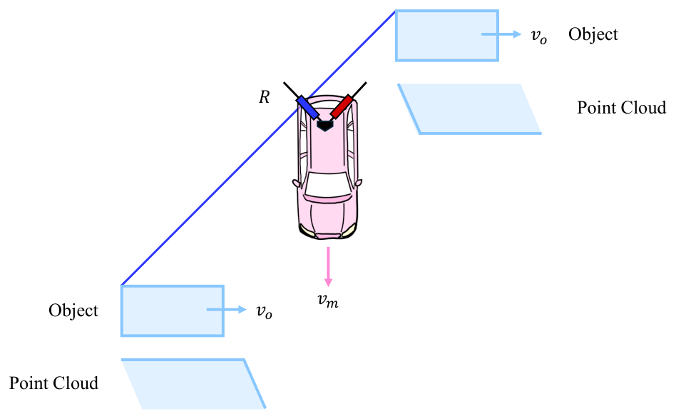
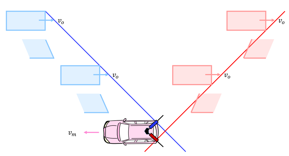
The same relative motion scanned from either side of the mapper produces identical distorted point clouds. — **The side does not matter.** Scanning from the left or right of the mapper gives the same distortion if the relative angle θ is the same.

Objects at increasing distances from the mapper produce point clouds with the same tilts, only farther apart. — **Distance does not matter.** Moving the object farther away only spreads the left and right clouds apart. The tilts stay the same.

Both follow from the equations: distortion depends only on the speeds, the direction of travel and the scanner angles. The simulator below lets you check this for yourself.

Common questions

Isn't this handled by motion compensation?

Standard compensation corrects for the scanner's own motion using GNSS and IMU data. That fixes static scenery but does nothing for an object with its own velocity. Correcting moving objects requires knowing, or estimating, how they moved. These equations describe exactly what that motion does to the cloud.

Is this the same as the rolling-shutter effect?

It is closely related. Both happen because a scene is captured over time rather than all at once. Rolling shutter usually refers to the sensor's own motion; here the subject is the motion of the objects being scanned, relative to a moving scanner.

Why does it matter in practice?

Vehicle dimensions extracted from MLS data can be wrong by metres, layover can put the front of a vehicle where its back should be, and skewed boxes confuse object detectors and change-detection pipelines. Knowing the distortion lets you predict it, flag it, or remove it. It also opens the reverse problem: estimating an object's speed from how distorted it looks.

What does the model assume?

Constant, straight-line velocities for both the mapper and the object; fixed scanner angles; flat ground; a single-channel 2D rotating scanner fast enough that each rotation is effectively instantaneous; and a rigid box-shaped object that does not rotate. Extending it to acceleration, turning objects and multi-beam 3D LiDAR is future work.

Interactive

Distortion explorer

Set the speeds and directions, then press Play scan. The drawing is a top-view simulation of a 4 m × 2 m box scanned by a tilted profile scanner. It is computed from the geometry alone, without the equations, so you can watch the distortion emerge and compare it with what the equations predict.

Thesis test cases:

Mapper speed v_m

Object speed v_o

Direction θ 0° = same direction as the mapper, 180° = head-on

Scanner

Horizontal angle φ_h

Vertical angle φ_v Affects β and α only (the top view is unchanged)

Point density

Display only: thins the drawn points, not the simulation

View

Scan-line speed v_lkm/h, signed

Scanned length l_s

Top tilt γtop face

Side tilt βside faces

Deviation αfront/back

Readouts use the paper's equations. Negative lengths mean layover. The signs of γ, β and α follow the paper's equations. The presets use the same speed ratios as the thesis test cases (km/h here, cm/s in the thesis), so the readouts match Tables 6.1 and 6.2.

Method

The equations

Take the x-axis along the mapper's direction of travel, y to its left and z up. The object moves at speed v_o at angle θ to the mapper, which moves at v_m. Both move in straight lines at constant speed.

Symbol	Meaning
v_m, v_o	Speed of the mobile mapper and of the object
θ	Angle between their directions of motion (0° same, 180° opposite)
φ_h, φ_v	Horizontal and vertical orientation angles of the scan plane
v_l	Speed at which the scan plane sweeps along the object's path
l_a, l_s	Actual length of the object and its length in the point cloud
γ, β, α	Tilt of the top face, tilt of the side faces, deviation of the front/back faces
τ	Included angle between front and side faces of the undistorted object (90° for a box)

1. How fast the scan plane sweeps the object's path

The first step turns the mapper's speed into the speed of the scan plane along the object's path:

v_{l} = \frac{v_{m} \cos φ_{h}}{\cos (θ \mp φ_{h})}

(1)

with − for the right scanner and + for the left. Read with its sign, v_l is positive when the sweep runs in the object's direction and negative when it runs against it. Its magnitude is what enters the equations below.

2. Length distortion

If the object moves against the sweep, the scan crosses it from front to back while the object closes the gap, so the cloud contracts:

Opposite directions

\frac{l_{s}}{l_{a}} = \frac{v_{l}}{v_{l} + v_{o}}

(2)

If they move the same way, the scan has to catch up:

Same direction

\frac{l_{s}}{l_{a}} = \frac{v_{l}}{v_{l} - v_{o}}

(3)

A negative ratio means the scan ran the wrong way through the object: layover. The cases follow directly.

Motion	Condition	Scan runs	Result	Point density
Opposite	any speeds	front → back	Contraction, l_s < l_a	higher
Same	v_l > v_o	back → front	Elongation, l_s > l_a	lower
Same	v_l = v_o	stays on one slice	Over-elongation, l_s = v_o t_s	lower
Same	v_o/2 < v_l < v_o	front → back	Layover elongation	lower
Same	v_l = v_o/2	front → back	Layover retention, \|l_s\| = l_a	unchanged
Same	0 < v_l < v_o/2	front → back	Layover contraction	higher

In over-elongation the cloud says nothing about the object's real size. Its length depends only on how long the scan lasted (t_s), so such points should be treated as outliers.

3. Parallelepiped distortion

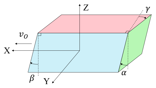
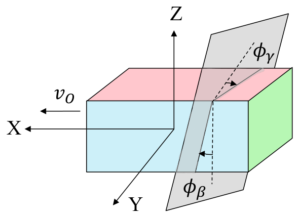
A cuboid point cloud distorted into a parallelepiped, with the top face tilted by gamma, the side face by beta and the front face deviating by alpha. — The three angles of a distorted box: γ (top), β (side), α (front/back).

A grey scan plane cutting a cuboid, with intersection angles phi-gamma on the top face and phi-beta on the side face. — Where the scan plane (grey) cuts the box: angles φ_γ on the top and φ_β on the side.

Each tilt is the plane's intersection angle with that face, scaled by how fast the object moves relative to the sweep, v_o,l (v_o − v_l in the same direction, v_o + v_l in opposite directions):

\tan γ = \frac{v_{o} \tan φ_{γ}}{v_{o, l}}, φ_{γ} = θ \mp φ_{h}

(4)

\tan β = \frac{v_{o} \tan φ_{β}}{v_{o, l}}, Φ_{β} = \cos^{- 1} (\frac{- \cos (φ_{h} - θ)}{\sqrt{\tan^{2} φ_{v} + \cos^{2} (φ_{h} - θ)}})

(5)

Φ_β comes from crossing the scan plane's normal with the side face's normal, and is then adjusted to φ_β by scanner side and θ (for the left scanner, φ_h is replaced by −φ_h). The two tilts together set the front/back deviation:

α = τ - \cos^{- 1} (\pm \sin γ \sin β)

(6)

with + for 0 ≤ θ < 180° − φ_h and − otherwise. When the sweep keeps pace with the object (v_l = v_o, same direction), the tilts become purely geometric: γ = φ_γ and β = φ_β.

The paper and thesis give the full derivations, the piecewise rules for each scanner, and summary tables for θ = 0°, 90° and 180°.

Results

Validation in simulation

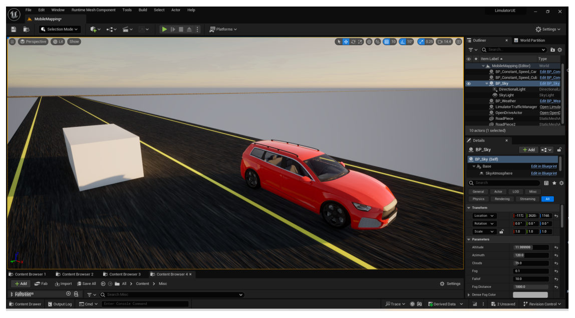
The equations were tested on synthetic LiDAR data from the SimDaaS simulation engine, built on Unreal Engine. The virtual mapper copies the StreetMapper-V system, which carries two RIEGL VQ-450 2D rotating scanners. A 4 m × 2 m × 1.5 m box drove past it in 17 test cases: five directions (0°, 40°, 90°, 130°, 180°) and a range of speeds. Some cases repeated a speed ratio with different absolute speeds, to show that only the ratio matters.

Unreal Engine scene with a red mobile mapping car and a white box on a road. — The simulated scene: the mobile mapper (red) and the moving box (white).

Simulation parameter	Value
Pulse repetition frequency	550 kHz
Channels	1
Scanning frequency	60 Hz
Wavelength	1.4 µm
Horizontal field of view	360°
Scan plane angles φ_h, φ_v	45°, 30°
Object (l × w × h)	4 × 2 × 1.5 m

Lengths and angles were measured on the simulated clouds in CloudCompare and compared with the predictions. Across all cases and both scanners, the root-mean-square errors were:

0.17 mLength l

0.57°Deviation α

0.49°Side tilt β

0.29°Top tilt γ

The remaining error comes from the data rather than the model. Points are sampled discretely, so corners and edges are never captured exactly, and the corner angles had to be measured by hand.

Show all length test cases (thesis Table 6.1)

Case	θ	v_o (cm/s)	v_m (cm/s)	Left obs.	Left pred.	Right obs.	Right pred.
A0	0°	0	400	4.00	4.00	4.00	4.00
A1	0°	200	400	8.08	8.00	8.08	8.00
A2	0°	400	400	–	–	–	–
A3	0°	1000	400	−2.67	−2.67	−2.66	−2.67
B1	180°	200	400	2.66	2.67	2.65	2.67
B2	180°	400	400	1.99	2.00	1.98	2.00
B3	180°	400	800	2.66	2.67	2.64	2.67
C1	90°	200	400	2.65	2.67	7.99	8.00
C2	90°	400	400	1.99	2.00	–	–
C3	90°	600	400	1.59	1.60	−7.97	−8.00
D1	40°	200	400	4.26	4.26	13.57	13.53
D2	40°	400	400	4.24	4.56	−9.75	−9.78
D3	40°	400	800	4.19	4.26	13.44	13.53
D4	40°	800	1000	4.43	4.44	−31.34	−31.48
E1	130°	200	800	2.37	2.96	4.20	4.13
E2	130°	400	400	1.96	1.66	3.93	4.56
E3	130°	800	400	1.02	1.05	5.27	5.31

Scanned lengths in metres; the true length is 4 m. Negative values are layover. “–” marks over-elongation, where the length grows with scan time. The angle results (Table 6.2) are in the thesis.

Limitations

The model assumes constant straight-line velocities, flat ground, a single-channel 2D scanner and a rigid object that does not rotate. Validation used simulation only, because public MLS datasets lack ground-truth velocities for moving objects. Natural next steps are non-uniform motion, multi-beam 3D LiDAR, estimating object velocity from the distortion itself, and correcting distorted clouds with these equations.

Resources

Read and teach

Journal articleJournal of Surveying Engineering (ASCE), 2026 · Editor's Choice
DOI
ThesisFull derivations, literature review, appendix tables for every case · IIT Kanpur, 2025
figshare
Defense slidesA visual walk-through of the problem and the derivations
Zenodo
Poster, GeodCon-26National Symposium on Geodesy, INSA New Delhi, 2026
figshare
Poster, Geospatial Technologies and Smart Cities WorkshopIIT Kanpur & University of Melbourne, 2025
figshare

Teaching with this page. The five-step primer and the explorer work as a self-contained lesson for surveying, remote sensing or robotics courses. One exercise: have students predict whether a case contracts, elongates or lays over, using only Equation (1) and the table, then check with the explorer.

Cite

BibTeX

If this work is useful in your research, please cite the paper:

@article{singh2026modeling,
  title   = {Modeling Point Cloud Distortions in Mobile Laser Scanning for Surveying},
  author  = {Singh, Aman Kumar and Lohani, Bharat},
  journal = {Journal of Surveying Engineering},
  volume  = {152},
  number  = {3},
  pages   = {04026006},
  year    = {2026},
  doi     = {10.1061/JSUED2.SUENG-1663}
}

and, for the full derivations, the thesis:

@mastersthesis{singh2025understanding,
  title  = {Understanding and Modeling Motion-Induced Point Cloud Distortions in Mobile Laser Scanning},
  author = {Singh, Aman Kumar},
  school = {Indian Institute of Technology Kanpur},
  type   = {B.Tech--M.Tech (Dual Degree) Thesis},
  year   = {2025},
  doi    = {10.6084/m9.figshare.32005947}
}

Acknowledgements

The thesis was supervised by Prof. Bharat Lohani. We thank Sourav Yadav and Manasvi Kale of SimDaaS for their support with the simulation environment. Figures are from the thesis.